


Insight in the testing methodology - Current


Mean, median and mode. All three of them are often mistakenly referred to as averages, whilst strictly speaking only the arithmetic mean, is an average. All three measures can be used to represent a dataset as a single number. The statistical term for these measures is the central tendency. This blog will explain the similarities and differences between these central tendency measures, and show which are used by GO-EUC in the researches that are done and why.
Statistics, the practice or science of collecting and analysing numerical data in large quantities, especially for the purpose of inferring proportions in a whole from those in a representative sample.
At GO-EUC data is collected in large quantities, for a typical scenario over 360 megabytes of raw data is collected in CSV format.
While that doesn’t seem like much data by todays standards, a single character using the default Windows UTF-16 encoding takes up 16 bits, or 2 bytes. This means that the 360MB, means of 188743680 characters. With a monospaced font in Word, 2176 characters fit on a default A4 page. This means that 86739 pages would be nessecary to print out all the data for one single GO-EUC scenario. The amount of paper needed to print out this amount of data would equal more than 1 complete tree! (source: https://science.howstuffworks.com/environmental/green-science/question16.htm)
In order to represent and compare this amount of data in a understandable, and easier to digest format, central tendency numbers are used at GO-EUC.
The definition of the three most commonly used central tendencies can be explained best with an example.
Take the following logon times in seconds for a given test. Let’s assume that the dataset is limited to these runs, and therefor 7 data points. For sake of argument these are all integer, or whole numbers.
| Run 1 | Run 2 | Run 3 | Run 4 | Run 5 | Run 6 | Run 7 |
|---|---|---|---|---|---|---|
| 9 | 10 | 9 | 15 | 11 | 9 | 10 |
With these results in the dataset, the mean is the total sum of all values in the dataset, divided by the number of values of the dataset, or:
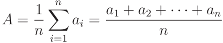
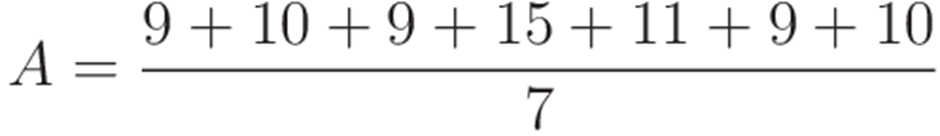
This represents the mean of the given data set, which in this case is 10.4, rounded down to 10.
With PowerShell, the Measure-Object cmdlet can be useed to calculate the mean of an given array:
$list = (9,10,9,15,11,9,10)
$mean = ($list |Measure-Object -Average).Average
write-host $mean
write-host ([math]::Round($mean))
In Python the built-in module statistics can be used to calculate the mean with the mean() function:
import statistics
list = [ 9,10,9,15,11,9,10]
mean = statistics.mean(list)
print(mean)
10.428571428571429
print(round(mean))
The mode is the value that appears most in the dataset, the most common value. From the data set listed above, a login time of 9 seconds appears 3 times and is therefore the mode of the data set is 9.
The mode is a little more cumbersome to calculate with Powershell:
$list = (9,10,9,15,11,9,10)

foreach ($group in ($list |group |sort -Descending count)) {
    if ($group.count -ge $i) {
        $i = $group.count
        $mode += $group.Name
    }
    else {
        break
    }
}
write-host $mode
In Python the statistics module can be used again, this time with the mode function:
import statistics
list = [ 9,10,9,15,11,9,10]
mode = statistics.mode(list)
print(mode)
Mode is most useful as a measure of central tendency when working with datasets categorical data, such as models of cars or flavors of soda, for which a mathematical average like the median value based on ordering is not possible to be calculated.
The median is the middle number in the list of data points, when ordered from smallest to largest. This means that half of our data set will be smaller than the median and half of the data set will be larger than the median.
To retrieve the median from the dataset, it first had to be ordered:
| dataset (ascending order) |
|---|
| 9 |
| 9 |
| 9 |
| 10 |
| 10 |
| 11 |
| 15 |
The middle number as shown above is 10, which means that in this dataset the median is 10.
As shown in the example, for a data set with an odd number of data points, the median is the middle number. If the data set were to have an even number of data points, the median would be the mean of the middle two number in the data set.
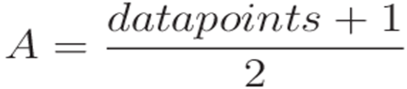
The middle number of the data set can be calculated as follows:
Using Powershell the median can be calculated as follows:
$list = (9,10,9,15,11,9,10)

#sort the list in ascending order
$list = $list | sort

#check if the list contains an odd or and even number of elements
if ($list.count%2) {
    #list containts an odd number of elements
    $median = $list[[math]::Floor($list.count/2)]
}
else {
    #list containts an even number of elements
    $Median = ($list[$list.Count/2],$list[$list.count/2-1] |Measure-Object -Average).average
}
Write-host $Median
Once again with Python the statistics module is leveraged which contains a function for the Median calculation as well:
import statistics
list = [ 9,10,9,15,11,9,10]
median = statistics.median(list)
print(median)
The arithmetic mean is most often used to report central tendencies, but it is not described as a robust statistic, meaning that it is greatly influenced by outliers. The median however is considered more robust against outliers. While outliers are not bad in principle, outliers could be considered as problematic, as they can potentially distort the results.
Outliers are values that are very much larger or smaller than most of the values in a given dataset. At GO-EUC we have to deal with outliers frequently.
Take for example a situation where in a given scenario CPU metrics have been collected for a single test run on a multisession VDI. It is expected that when the VDI is loaded with virtual users that the VDI’s CPU usage will start to increase. At certain points in the scenario there are bound to be spikes in the CPU usage, sometimes even as high as 100%. For this frame of reference, these spikes are considered to be normal behavior and are just part of the dataset.
Other times due to faults in the measuring or other outside influences out or our control, the data set can contain outliers that are not expected. These outliers can influence the averages, the arithmetic mean of the dataset. In the login time dataset example used above, it is assumed that 15 is a correct value, but this could also be an error in the measurements taken. The mean in this case is affected by this perhaps false measurement. This example can be taken even further; what if one of the Loadgen servers which are used to feed the VDIs with simulated users was in a faulty state which caused the logins initiated from this server to take excessively longer than expected and thereby greatly influencing the average login times.
There are several ways to handle these outliers. The most commonly used method at GO-EUC is to leave the identification of these outliers to the analysts and strip these abnormal or faulty measurements from the dataset before we calculate the averages (the mean) that are reported in the final publication. However, this method can be combined with a more scientific method. This could for instance be to use a percentile based approach, for example using the 95th percentile and include this in the measurements that are to be reported on.
Let’s take a slightly larger data set for this example. Below is a table with CPU usage data collected from a given run:
| CPU Usage in % |
|---|
| 17 |
| 16 |
| 9 |
| 6 |
| 3 |
| 26 |
| 17 |
| 33 |
| 8 |
| 10 |
| 7 |
| 13 |
| 1 |
| 5 |
| 22 |
| 42 |
| 4 |
| 25 |
| 14 |
| 12 |
| 24 |
| 23 |
| 20 |
| 5 |
| 22 |
| 56 |
| 28 |
| 11 |
| 18 |
| 21 |
56 seems to be the obvious outlier here. Without any calculation we might conclude that leaving 56 out, the outliers will have been eliminated. By calculating the 95th percentile this assumption can be evaluated. In order to calculate the 95th percentile the total number of values in the dataset, in this case 30 is represented by N and as such N=30. To calculate the 95th percentile multiply N with 30 to get 28,8.
After we’ve sorted the list in ascending order:
| CPU Usage in % (ascending order) |
|---|
| 1 |
| 3 |
| 4 |
| 5 |
| 5 |
| 6 |
| 7 |
| 8 |
| 9 |
| 10 |
| 11 |
| 12 |
| 13 |
| 14 |
| 16 |
| 17 |
| 17 |
| 18 |
| 20 |
| 21 |
| 22 |
| 22 |
| 23 |
| 24 |
| 25 |
| 26 |
| 28 |
| 33 |
| 42 |
| 56 |
In the ordered list 95th percentile is 29. Now leaving the values from the ordered dataset greater than 29, the dataset will exclude 42 and 56, Because these values fall out of the 95th percentile, these values will be discarded from the dataset. By looking at the 95th percentile, both 42 and 56 are considered outliers.
While statistically correct, just removing these values from the dataset without proper inspection would be short-sighted or at least a too simplistic approach. In order to properly assess if the outliers can be safely removed, we need to carefully look at the data, at what we want to measure and take all factors into consideration in order to determine if these values are indeed ‘polluting’ our dataset and need to be removed. The tradeoff is that the removal will inherently cause some loss of information.
Sometimes not only the top outliers, but also the bottom outliers need to be evaluated and for this we can also calculate the 5th percentile. Trimming both the top and bottom 5 percentages of the data will result in a truncated mean. The truncated mean is also a measure of central tendency, just like the ‘normal’ mean and the median. The truncated mean is calculated as a mean after trimming the outliers at the high and the bottom end of the dataset. One thing to bear in mind is that by using the truncated mean more information was removed from the original dataset.
The truncated mean is sometimes erroneously referred to as the Winsor mean. With the Winsor mean however, the data is not trimmed, but the dataset is altered or censored because with winsorizing the outliers are, in contrast to the truncated mean, replaced by certain percentiles.
The metrics and data collected by GO-EUC should be able to give an valuable insight to the readers.
GO-EUC still uses the most commonly used central tendency, the mean, for summarizing data sets most of the time. Because the majority, if not all, of the data collected is of an ordinal nature, the mode is not useful for our researches. The median however is considered valuable measure and at GO-EUC we will see how we can report the median of the datasets in our future research.
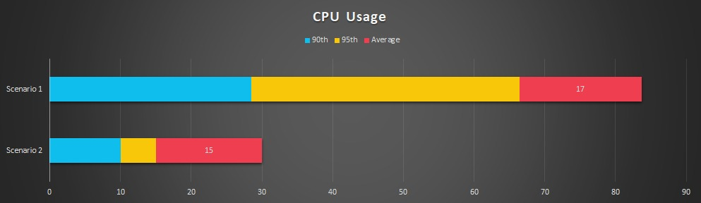
As for handling outliers, when considering removing data points that are considered outliers, we’ll calculate the 95th percentile and use that value to identify the outliers before removing these values from the data sets that will be reported on in the coming future. This means that the presentation of the data could also change, as shown in the chart below. Here we have to scenarios, and the bar chart for both scenarios not only shows the mean, but also the 90th and 9th percentile.
Here, the percentile values are incorporated into the bar chart. The average or mean is still the primary statistic that we report, but it is complemented with the percentile values from the dataset.
Dealing with central tendency and outliers in data isn’t as clear cut as it seems on the surface. Relying only on perception when it comes to dealing with outliers or completely relying on math, both don’t do the data justice. By combining several methods mentioned in this blog post, we can not only see when and if the data that is collected is imbalanced, but also where the data is deviates from the (expected) norm. Detecting and classifying outliers is an integral part of the data analysis performed and involves in-depth knowledge on all the variables of the tests.
At GO-EUC we always strive for statistical accuracy for, and reproducibility by the community. Our goal is always to show the best best possible representation of the datasets used in our researches.
We hope this was informative and has given some deeper insight on central tendency and our way of working with data.
If you have any questions or comments around statistics or any other topics around performance and scalability, please don’t hesitate to reach out to us on social media (twitter/linkedin) or join the World of EUC Slack channel!
Photo by Mika Baumeister

Echteld, Netherlands

Malta